Summary of Key Quantum Ideas
A wavefunction provides the complete description of a quantum state. In order to determine different qualities of a wavefunction an operation must be performed. Operating on wavefunction yields an observable, or a value specific to that quantum state. Different operators provide different information - there are operators for position, momentum, energy, etc.
Functions as eigenfunction
An operator performs a certain operation on a function. As we’ve previously mentioned, this could range from multiplying a function by a variable, like the position operator, or taking the second derivative of a function, like the Hamiltonian operator. Operators can only operate on functions which are eigenfunctions for the operator. For a wavefunction to be an eigenfunction of an operator, the operation must return the original function multiplied by a scalar multiple. This scalar multiple is the eigenvalue of that operator and the observable value that we are trying to find.
More concisely put:
\begin{equation}\label{help}{\hat{O}}{\psi}=\lambda_i{\psi}\end{equation}
Where ${\hat{O}}$ is an operator, ${\psi}$ is an eigenfunction, and ${\lambda}$ is an observable.
The Hamiltonian operator operating on an eigenfunction will yield the energy of that quantum state multiplied by the original eigenfunction:
$ \hat{H}\Psi = {E}\Psi $
The Hamiltonian operator combines the potential energy of a certain quantum state with the kinetic energy of a state, and this operation can be done using calculus:
$ \hat{H} = \frac{-\hbar^2}{2m}\frac{\partial^2}{\partial x^2} + {V(x)} $
This expression is also called the Time Independent Schrodinger Equation. Note that this expression only depends on position, not time.
-
The solutions to the Schrodinger, or the set of eigenvalues can be represented by $ {E_n} $. This set is the complete list of possible total energy measurement results.
-
If two operators do not commute, then they do not share the same set of eigenfunctions. This is also to say that they do not have the same basis.
All operators we use are hermitian
Hermitian operators produce real eigenvalues.
How can the energy of a quantum state be determined?
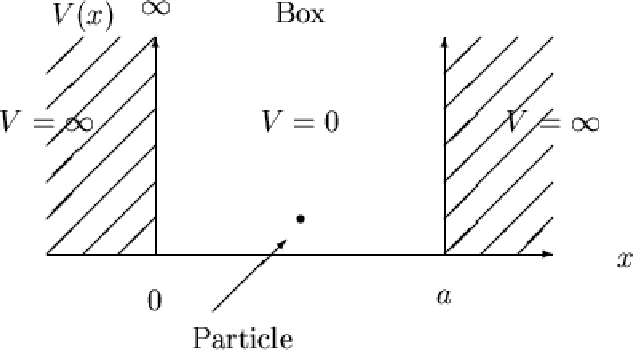
The Hamiltonian operator is composed of both the kinetic energy and potential energy operator. In simplified models, like the one-dimensional particle in a box model, the potential energy of the box is generally set to zero while there is infinite potential energy out of the box - this is to say that the particle exists in a well of infinite potential.
Linear Algebra Translation
Operators as Matrices
Operators now become matrices when using linear algebra to gain information about quantum states. The expression above can be modified slightly:
\begin{equation}\label{merp} \mathbf{O}\vec{v_i}=\lambda_i \vec{v_i} \end{equation}
Where ${O}$ is a matrix, ${v}$ is an eigenvector, and ${\lambda}$ is the observable.
All operators we use are hermitian
A hermitian matrix has a defining property where the complex conjugate is equal to the complex conjugate transpose. A complex conjugate transpose is the original matrix with the rows now serving as the columns and the columns serving as the rows, and any complex components of the matrix are replaced with $ -i = -\sqrt{-1} $.
Eigenfunctions = Eigenvectors
Vectors can now be used to hold the same information that eigenfunctions hold. The basis of a vector will matter, and choosing to express a vector in a different basis has the potential to simplify the vector. For example, if the energy of the second eigenvector of the particle in a box model is found and presented in the energy basis, the vector would be:
$ {\vec{v}}=\begin{bmatrix} 0 \\ 1 \\ 0 \\ \vdots \end{bmatrix} $
This vector suggests that only the second eigenvector is contributing to the overall state.
Quantum states are linear combinations of states
In the linear algebra representation of quantum states, different vectors combine to form each eigenstate. Here’s a graphical representation of this concept, where vector $\vec{w}$ can be written as a linear combination of vectors $\vec{u}$ and $\vec{v}$:
This concept is depicted more generally by this equation, where the ${c}$ refers to the coefficient, or the contribution of each vector state, ${p}$, to the overall state, ${\vec{v}}$:
\begin{equation}\label{hey} \vec{v} = c_1\vec{p_1} + c_2\vec{p_2} + c_3\vec{p_3} + … + c_n\vec{p_n} \end{equation}
Inner product vs. Matrix multiplication
We will use both operations to manipulate our matrices and vectors, but the inner product of two vectors is quite different than the multiplication of two vectors. For our purposes, we are considering column or row vectors.
The inner product is the sum of each entry in one vector multiplied by the corresponding entry of a different vector. This manipulation results in a scalar. To get the inner product, a row vector is multiplied by a column vector, and these two vectors must have the same number of entries.
$ \text{inner product} ={\begin{bmatrix} v_{1} & v_{2} & … & v_{n} \end{bmatrix}}^* \begin{bmatrix} u_{1} \\ u_{2} \\ \vdots \\ w_{n} \end{bmatrix}=\sum_{n=1}^{n}v_i ^*u_i $.
When two vectors are multplied, a new square matrix of the same dimensions (if the two vectors have the same number of entries) is generated with each entry in this new vector being the product of the corresponding entries of the two initial vectors. This outer product is generated by multiplying a column vector by a row vector. The order of this multiplication does matter.
$ \text{outer product} = \begin{bmatrix} u_{1} \\ u_{2} \\ \vdots \\ u_{n} \end{bmatrix}^* {\begin{bmatrix} v_{1} & v_{2} & … & v_{n} \end{bmatrix}} = \begin{bmatrix} u_{1}* v_{1} \\ u_{2}* v_{2} \\ \vdots \\ u_{n} * v_{n} \end{bmatrix}$
Vector Normalization
We want to work with vectors which have a length of 1 - this is to say that the vector is normalized. We can normalize a vector by dividing that vector by its own length: \begin{equation} \vec{v_n} = \frac{\vec{v}}{\parallel\vec{v}\parallel} \end{equation}
Hamiltonian operator as a matrix
Using linear algebra, we can construct a matrix that will similarly take the second derivative of another matrix within the context of the Particle in a Box problem. We can then combine this kinetic energy matrix with the potential energy to form the Hamiltonian operator in the form of a matrix. The potential energy is characteristic of the system in which the particle exists.
Here, we create a vector of zeros with the first three and last three entries (as w=3) equal to the height of our potential energy well to model that the potential energy of our system goes to infinity at the edge of our box. By putting this vector on the diagonal of a new matrix, V, we’ve created the potential energy matrix.
Vvec = zeros(pts, 1)
Vvec([1:w, end - (w-1):end]) = barht;
V = diag(Vvec);
We’ve then created a matrix which will find the kinetic energy of a different matrix. The second derivative of a function can be thought of as how the change in slope of a graph changes, and a similar thought is used here to consider how the change in entries of a vector change. This second derivative matrix shown below is then multiplied by 1/dx^2 and that resulting matrix is then multiplied by frac{/hbar^2}{2* m} to determine the total kinetic energy of the vector.
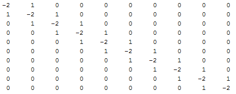
D2 = (1/(dx^2))*(-2*eye(pts) + diag(ones(pts-1,1), 1) + diag(ones(pts-1,1),-1));
T = (-hbarsq/(2*m))*D2
The Hamiltonian matrix consists of both the potential energy matrix and the kinetic energy matrix.
H = T + V;