home

Particle in a Box

The particle-in-a-box model builds from one dimensional motion to three dimensional motion, and restricts the movement of a particle by certain boundary conditions. This model is said to mimic the idealized movement of a gas-phase molecule that is free to move in a container. If there are no boundary conditions, the particle acts as a free particle and can exist anywhere. With the addition of boundary conditions, the function is only allowed to exist at certain positions - this is to say that we have quantized our particle’s movement. We model the particle’s movement with a function, called a wavefunction, and can use mathematical operations to describe many properties of the particle. The particle’s motion can also be thought of being modeled by a wavevector, and thus the Particle in a Box model also lends itself to linear algebra applications as well.

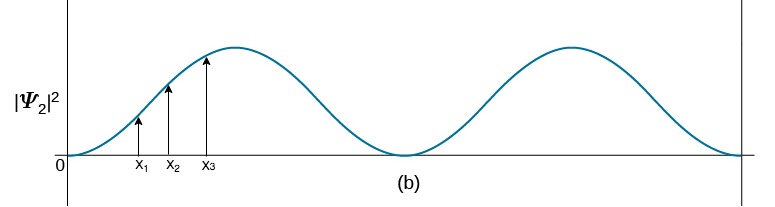
By placing the particle in a box surrounded by infinite potential, the particle essentially can only exist within the box, and therefore the motion is constrained. This simple model illustrates the foundation of quantum mechanics and quantization of energy. While theoretically, the particle’s motion is constrained by impenetrable walls of potential energy, in reality, particles have the ability to tunnel through potentials which they would not classibly be able to penetrate. Quantum tunneling is the phenomenon of particles overcoming energy potentials that these particles do not classically have the capability to overcome. The energy that the particle needs to overcome the barrier is higher than the energy of the particle, therefore, following the classical laws of physics, the particle would not be able to change state. This tunneling phenonmenon can be observed in the figure below, where the probability amplitude of the particle is first plotted (a) and then the probablity density is displayed (b):

From: http://sdsu-physics.org/physics197/phys197.html

The second energy eigenfunction of the Particle in a Box model in the position basis can be thought of as a linear combination of different ${x}$ positions to create an overall function. The ${x_1}$ position has some contribution to the overall function, the ${x_2}$ position has a different contribution to the overall function, and the ${x_3}$ position has a different contribution to the overall function. This idea continues for all ${x}$ positions and their contributions, and therefore an overall quantum state. The figure simplifies this concept by spacing out the ${x_1},{x_2},$ and ${x_3}$ positions, but these positions can be thought of as infinitely close.

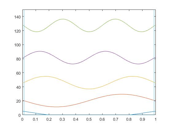
We’ve created a program which discritizes space and combines the potential energy and kinetic energy into a PIB hamiltonian matrix. The eigenvalues and eigenvectors of this matrix have also been determined and sorted in two different matrices. One is a matrix composed of the sorted eigenvectors. The eigenvalues of the total energy matrix are the diagonal elements of another matrix, vals. Once the eigenvalues and eigenvectors of the Hamiltonian matrix were found, these eigenvalues and eigenvectors were sorted so that they will be plotted in the correct order. The graphs of each eigenvector were then shifted upwards and scaled so that they could be seen more easily.

This is the code which sets the length of the box, the mass of the particle, and $ \hbar^2 $ and produces a figure containing $ n $ number of eigenvectors for the one dimensional PIB, spaced according to their energies.

---

Code from Matlab to plot the eigenvectors of the PIB model

function [x,E,psiX,psiE]=TDSE

First a number of different constants must be defined. Here, the mass of the particle (m), the length of the box (L), and ${\hbar^2}$ are all defined as 1 in order to simplify the problem. The height of the barrier is defined as a large number to account for the infinite potential of the box and is set at ${1 x 10^6}$. A new variable w is defined as 3 in order to construct the potential wall, where w is essentially the width of the barrier. The number points used is set equal to 250.

%here are my constants: %m is mass, L is length of box, barht height of barrier, w is the barrier width
m = 1;
L = 1;
hbarsq = 1;
barht = 1e6;
w=3;
pts = 250;

The number of elements in the x vector is now defined. The linspace command is used to create a vector of x values which span from zero to the box length and are composed of pts number of elements. These x elements are evenly spaced between 0 and L. The change in x between all of these points is constant, as the points are evenly spaced and defined here as the difference between the second x element and the first x element.

%now account for the delta x and discritize the number of elements in the x vector
x = linspace(0, L, pts)';
dx = x(2)-x(1);

The potential vector ${Vvec}$ can now be constructed by creating a vector of zeros. This defines the potential energy within the box to zero, and by setting the first and last three entries of the barrier equal to the ${barht}$ defined above, a well with infinite potential is created.

%x is a vector that goes from 0 to L separated by some amount, dictated by the number
%of points. Vvec is a vector with the dimension of pts entries with one column
% now we have points number of entries in the x vector
Vvec = zeros(pts, 1);
Vvec([1:w, end - (w-1):end]) = barht;
%Vvec(120:130) = 75;
%this makes a barrier in the middle of the box

By putting the entries of Vvec on the diagonal of a new matrix, V, the potential energy matrix has been created.

%Now we create the potential energy matrix but putting the entries of Vvec in a diagonal matrix

V = diag(Vvec);

We’ve then created a matrix which will find the kinetic energy of a different matrix. The second derivative of a function can be thought of as how the change in slope of a graph changes, and a similar thought is used here to consider how the change in entries of a vector change. This second derivative matrix shown below is then multiplied by ${1/dx^2}$ and that resulting matrix is then multiplied by $\frac{\hbar^2}{2* m}$ to determine the total kinetic energy of the vector.

%making the second derivative matrix
D2 = (1/(dx^2))*(-2*eye(pts) + diag(ones(pts-1,1), 1) + diag(ones(pts-1,1),-1));
%now account for the delta x idea by subtracting the first element from the second element because they will be evenly spaced, and multiply the matrix by the constants 
T = (-hbarsq/(2*m))*D2;

A new matrix H is then defined as the sum of the potential energy matrix and the kinetic energy matrix, as the Hamiltonian takes both the potential energy and kinetic energy in account in order to solve the total energy of a state.

%here's our Hamiltonian, which accounts for both the potential energy and kinetic energy

H= T + V;

The [vecs, vals] command creates two new matrices which are the eigenvectors and eigenvalues of the matrix, H. The vecs matrix has the eigenvectors of H as columns in the matrix, and the vals matrix has all of the eigenvalues for H on the diagonal of the matrix.

%now we want to solve for the eigenvalues of the square matrix H

[vecs, vals] = eig(H);

The srtvecs commmand, described here puts the eigenvectors and eigenvalues together in ascending order of energy level.

%now we sort the vectors and values so that they are plotted in ascending order of n, but the eigenvalues and eigenvectors stay together
[srtvecs, srtvals] = eigsort(vecs, vals);

Each energy level graph will then be shifted up by their own energies so that these different energy levels can be better visualized. A new matrix, called repvals, will be used in order to shift up the graphs. This shift must also be scaled by a factor in order for it to be better visualized. The shiftvecs matrix is a new matrix where the entries of the shifted eigenvectors have each been shifted up by their corresponding energy eigenvalue.

%now we will need to shift the graphs up so that they are on different levels 
%start to make the repvals matrix, where k is a vector composed of the diagonal components of the vals matrix and l is a vector with points rows and one column

k = diag(srtvals);
l = ones(pts, 1);
%k becomes k' so that the dimension matches such that we get a matrix of our eigenvalues. 
repvals = l*k';
%defining shiftvecs so that the graphs will be shifted up. Shiftvecs must also be scaled by some factor to make it easier to visualize
sc = 100; 
shiftvecs = repvals + sc*srtvecs;

The resulting eigenvectors which have been shifted up by their energies are then plotted with the potential well also plotted on the same graph.

%we need to create a vector which has the diagonal entries of the potential energy matrix
v = diag(V);


figure (1); plot(x, shiftvecs(:,1:n), x, v)

shiftvecs = shiftvecs(:,1:n);

axis([min(x) max(x) min(v) 1.1*max(max(shiftvecs))])

end

home