home

Particle in a Box Code

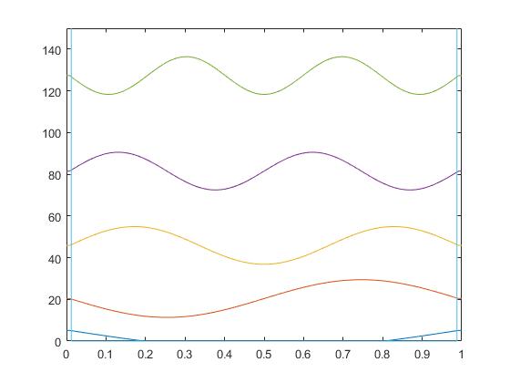
We’ve created a program which discritizes space and combines the potential energy and kinetic energy into a PIB hamiltonian matrix. The eigenvalues and eigenvectors of this matrix have also been determined and sorted in two different matrices. One is a matrix composed of the sorted eigenvectors. The eigenvalues of the total energy matrix are the diagonal elements of another matrix, vals. Once the eigenvalues and eigenvectors of the Hamiltonian matrix were found, these eigenvalues and eigenvectors were sorted so that they will be plotted in the correct order. The graphs of each eigenvector were then shifted upwards and scaled so that they could be seen more easily.

This is the code which sets the length of the box, the mass of the particle, and $ \hbar^2 $ and produces a figure containing $ n $ number of eigenvectors for the one dimensional PIB, spaced according to their energies.

---

Code from Matlab to plot the eigenvectors of the PIB model

function plotPIB1D (n)

%n refers to the number of eigenvectors generated

%here are my constants: 
%m is mass, L is length of box, barht height of barrier, w is the barrier
width 

m = 1;

L = 1;

hbarsq = 1;

barht = 1e6;

w=3; 

pts = 250;


%now account for the delta x and discritize the number of elements in the x vector 

x = linspace(0, L, pts);

dx = x(2)-x(1);

%x is a vector that goes from 0 to L separated by some amount, dictated by the number of points. Vvec is a vector with the dimension of pts entries with one column. now we have points number of entries in the x vector

Vvec = zeros(pts, 1

Vvec([1:w, end - (w-1):end]) = barht;

%We created a vector of zeros, but we just set the first three and the last three entries (because w=3) equal to some barht (large number, using 1e6) to model the infinite potential well


%Now we create the potential energy matrix but putting the entries of Vvec in a diagonal matrix

V = diag(Vvec);

%making the second derivative matrix

D2 = (1/(dx^2))*(-2*eye(pts) + diag(ones(pts-1,1), 1) + diag(ones(pts-1,1),-1));

%now account for the delta x idea by subtracting the first element from the second element because they will be evenly spaced, and multiply the matrix by the constants 

T = (-hbarsq/(2*m))*D2;


%here's our Hamiltonian, which accounts for both the potential energy and kinetic energy

H= T + V;

%now we want to solve for the eigenvalues of the square matrix H

[vecs, vals] = eig(H);

%now we sort the vectors and values so that they are plotted in ascending order of n, but the eigenvalues and eigenvectors stay together

[srtvecs, srtvals] = eigsort(vecs, vals);


%now we will need to shift the graphs up so that they are on different levels 

%start to make the repvals matrix, where k is a vector composed of the diagonal components of the vals matrix and l is a vector with points rows and one column

k = diag(srtvals);

l = ones(pts, 1);

%k becomes k' so that the dimension matches such that we get a matrix of our eigenvalues. 

repvals = l*k';

%defining shiftvecs so that the graphs will be shifted up. Shiftvecs must also be scaled by some factor to make it easier to visualize

sc = 100;

shiftvecs = repvals + sc*srtvecs;

%we need to create a vector which has the diagonal entries of the potential energy matrix

v = diag(V);

figure (1); plot(x, shiftvecs(:,1:n), x, v)

shiftvecs = shiftvecs(:,1:n);

axis([min(x) max(x) min(v) 1.1*max(max(shiftvecs))])

end

home