home

An Introduction to Perturbation Theory

Perturbation theory is the idea that we can better understand the behavior of an unknown quantum state by first looking at a familiar, known model.

We’ve begun with a small introduction to perturbation theory with the left well/right well example. To better understand the behavior of the particle in the well with a central barrier, we can combine the behavior of the particle in the left well and right well. We will essentially change basis from the left well and right well to the basis of the central barrier. This mechanism will be further explored in the Perturbation2018 code presented below.

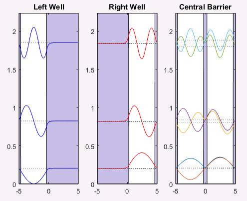
The vectors from the left and right well are contributing differently to the depiction of the central barrier, as depicted in the graphical representation below.

We can use these depictions of the right well and left well contributions to the central well to better understand the molecular orbital model of a H2 molecule. The one electron from each hydrogen atom can combine in the bonding sigma orbital, representative of constructive interference, or in the sigma star, or anti-bonding orbital representative of destructive interference between the two.

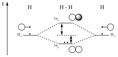
By analyzing the contributions of the left well and right well programs above to the overall central barrier picture, we can apply this new understanding to the ways in which hydrogen atomic orbitals combine during bonding events. As an introduction to the pertubation theory, in which one uses a known model or foundation to better understand an unknown model, we have developed a better understanding of the contributions of separate atomic orbitals to molecular orbitals by using this simplified left-well/right-well program.

function      Perturb2018
%% PIB example demonstrating the use of the eigenvectors of a simple hamiltonian to understand those of a more complicated one.

%% Define parameters
    v = 6;                                 % number of states to plot per well
    b = 10;                                % central barrier height
    hw = 2;                                % barrier half-width
    
    pts = 100;                             % number of spatial grid points
    x = linspace(-5,5,pts)';               % discretize space
    dx = x(2)-x(1);                        % space step
    hbar = 1;                              % Dirac's constant
    m = 1;                                 % particle mass

%% Compute Laplacian matrix; boundary conditions = 0
    D2 = -2*eye(pts)+diag(ones(1,pts-1),1)+diag(ones(1,pts-1),-1);
    D2 = D2/(dx^2);
    
%% Define three potential energy functions as vectors, then combine vectors into one 3-column matrix for ease of use.

    Vvec=zeros(pts,3);  % start with all zeros, 3 cols
    Vvec([1:3, round(pts/2)-hw:pts],1) = b; % change first col to create left well
    Vvec([1:round(pts/2)+hw, pts-3:pts],2) = b; % change 2nd col to create right well
    Vvec([1:3, round(pts/2)-hw : round(pts/2)+hw, pts-3:pts] ,3) = b; % change 3rd col to create central barrier

%% Define a consistent order in which colors are used for wavefunction plots.
    clrOrder = ['b' 'r' ' ']; % color order for plots; auto color for third plot
    
%% Bring up a figure window and clear it.    
    figure(1);% bring up and clear figure window   
    clf;
    
%% Compute energy eivenvectors for each PIB variation and plot them. 

for  well = 1:3
    V = diag(Vvec(:,well));  % make matrix with selected potential energy as diagonal
    H = -(hbar^2/(2*m))*D2 + V;			% Hamiltonian = potential + kinetic energies

% Calculate the eigenvectors and eigenvalues, then sort them
   [vecs,vals] = eig(H);
   [vecs,vals] = eigsort(vecs,vals);
   VECS(:,:,well) = vecs;   % store vecs as page in array
   vvals =  diag(vals) ;    % extract eigenvalues from vals in form of vector

% Add eigenvalues to eigenvectors to displace them vertically in prep. for plotting
   mvals = (vvals(1:v)*ones(1,pts))';    % create matrix with repeated eigenvalues as columns
   plotvecs = mvals+vecs(:,1:v);    % add v_th eigenvalue to v_th eigenvector to displace it vertically
                  
    subplot(1,3,well)
    area(x,diag(V));
    alpha(0.3);
    hold on
    plot(x,diag(V),'k',...   % plot V(x) in black
         x,plotvecs,clrOrder(well),...   % plot modified eigenvectors
         x,mvals,'k:')    % plot dotted lines as baselines for  plots
% Add titles to plots     
     if well==1
         title('Left Well')
     elseif well==2
         title('Right Well')
     else 
         title('Central Barrier')
     end
end
hold off

%% Set axis limits for each plot sequentially.
for j = 1:3
    subplot(1,3,j)
    axis([min(x) max(x) min(diag(V)) 1.1*max(max(plotvecs))])% set axes
end 

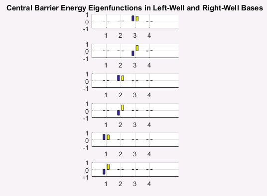
%% Create basis conversion matrices using left-well and right-well eigenvectors.
    EtoXL = VECS(:,:,1); % From energy to left-well basis conversion matrix
    XtoEL = inv(EtoXL);  % From left-well basis to energy conversion matrix

    EtoXR = VECS(:,:,2); % From energy to right-well basis conversion matrix
    XtoER = inv(EtoXR);  % From right-well basis to energy conversion matrix

    psiL = XtoEL*VECS(:, [1:2.*v], 3); % E eigenvectors in left-well basis
    psiR = XtoER*VECS(:, [1:2.*v], 3); % E eigenvectors in right-well basis

%% Reexpress central barrier stationary states using left-well and right-well eigenvectors as bases.
    figure(2)
    clf 
    indmax = 4;    % truncate E space plots to clarify display
for j = 1:v

    subplot(v,1,v-j+1)
    % plot expansion coeffs 1->indmax
    bar3([psiL(1:indmax,j) psiR(1:indmax,j)] ,0.5,'grouped')  % make a 3D bar plot
    view(-90,0)    % fix the view angle
    pbaspect([1 6 1])  % fix the plotting aspect ratio
    set(gca,'XTick',[1 5 10 15])    % show fewer tick marks
    
    if j==v
        title('Central Barrier Energy Eigenfunctions in Left-Well and Right-Well Bases')
    end
end