home

Modeling the Morse Potential

The Morse potential more accurately describes how the potential energy of a system changes with increasing internuclear distance. The Morse potential also models the plateau in potential energy at increasing distances, as the nuclei and electrons are no longer interacting if the distance between them is large. We’ve used a similar approach to model the allowed transitions between energy levels, but in order to model the selection rules with the Morse potential, we’ve defined the potential energy of the system as the Morse potential energy.

First, the time independent Schrodinger equation will be solved using the Morse potential to define our potential energy. The original particle in a box code was modified such that the potential energy matrix modeled the harmonic oscillator potential energy. Then the eigenvectors and eigenvalues can be solved. We will use the dipole moment as the transition operator to determine whether or not the transition is allowed. We say that the transition dipole operator is the complex conjugate of the final wavevector state multiplied by the x position multiplied by the initial wavevector. We yield a scalar which is proportional to the likelihood of the transition from one initial state to a final state. Therefore, the likelihood of the transition is equal to $\langle \psi_i | \mu | \psi_f \rangle$

The dipole transition operator is represented with $\mu$.

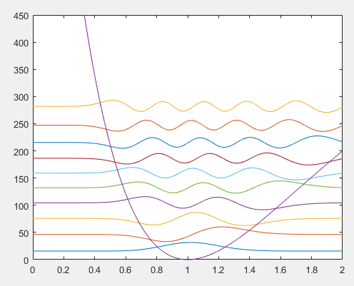
The plot of the Morse potential with the first ten energy levels is shown below.

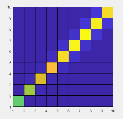
Below, the likelihood of the transition is depicted below using a color scale from blue to yellow. The It is expected, however, that the simple harmonic oscillator selection rules would hold at lower energies. For lower energy transitions, it is expected that transitions where the change in n is equal to 1 would be allowed. This idea, however, does not appear on the graphical depiction of the likelihood of transition below. There may be a problem with the code.

---

Matlab Code

First a number of different constants must be defined. Here, the mass of the particle (m),the charge (q), De, a, and ${\hbar^2}$ are all defined as 1 in order to simplify the problem. K refers to the spring constant in the problem. The number points used is set equal to 250. With n defined as one, the first 10 energy levels are plotted.

function morse(n)
    m = 1;
    hbarsq = 1; 
    pts = 250;
    k = 1e3;
    q = 1;
    n=10;
    De = 500;
    a = 1;
    

The number of elements in the x vector is now defined. The linspace command is used to create a vector of x values which span from zero to the box length and are composed of pts number of elements. These x elements are evenly spaced between 0 and L. The change in x between all of these points is constant, as the points are evenly spaced and defined here as the difference between the second x element and the first x element.

x = linspace(0, 2, pts);
dx = x(2)-x(1);

The potential vector Vvec can now be constructed with the potential energy of the Morse potential. By putting the entries of Vvec on the diagonal of a new matrix, V, the potential energy matrix has been created.

Vvec=De*(1-exp(-a*(x-1))).^2;
V=diag(Vvec);

We’ve then created a matrix which will find the kinetic energy of a different matrix. The second derivative of a function can be thought of as how the change in slope of a graph changes, and a similar thought is used here to consider how the change in entries of a vector change. This second derivative matrix shown below is then multiplied by ${1/dx^2}$ and that resulting matrix is then multiplied by $\frac{\hbar^2}{2* m}$ to determine the total kinetic energy of the vector. A new matrix H is then defined as the sum of the potential energy matrix and the kinetic energy matrix, as the Hamiltonian takes both the potential energy and kinetic energy in account in order to solve the total energy of a state.

 D2 = -2*eye(pts) + diag(ones(pts-1,1), 1) + diag(ones(pts-1,1),-1);   
 T = 1/(dx^2)*(-hbarsq/(2*m))*D2;
 H=T+V; 

The [vecs, vals] command creates two new matrices which are the eigenvectors and eigenvalues of the matrix, H. The vecs matrix has the eigenvectors of H as columns in the matrix, and the vals matrix has all of the eigenvalues for H on the diagonal of the matrix. The srtvecs commmand, described here puts the eigenvectors and eigenvalues together in ascending order of energy level.

[vecs, vals] = eig(H);
[srtvecs, srtvals] = eigsort(vecs, vals);

Each energy level graph will then be shifted up by their own energies so that these different energy levels can be better visualized. A new matrix, called repvals, will be used in order to shift up the graphs. This shift must also be scaled by a factor in order for it to be better visualized. The shiftvecs matrix is a new matrix where the entries of the shifted eigenvectors have each been shifted up by their corresponding energy eigenvalue.

k = diag(srtvals);
l = ones(pts, 1);
repvals = l*k';

sc = 100;
shiftvecs = repvals + sc*srtvecs;

The new variable transitions defines the probability of the transition by multiplying the vecs by the transition dipole operator by vecs again as described above. The result is a scalar which defines the probabiltiy of the transition. The probabilities of these transitions can then be plotted.

transitions=vecs'*(q*diag(x))*vecs;

    figure(1);pcolor(abs(transitions(1:n,1:n).^2))
    axis square
    figure(2);plot(x,shiftvecs(:,1:n),x,Vvec); 
axis([-inf inf 0 450]);
end