Fourier Transforms Introduction
The Fourier transform classically refers to the idea of tranforming a function which exists in time space into a function which exists in frequency space. A function of time can be transformed into a function of frequency, using the Fourier transform.
Generally, the Fourier transform can be expressed as:
The first equation allows for the transformation from the time domain to the frequency domain, while the second equation is the inverse Fourier which allows for the transformation from the frequency domain to the time domain.
Position and Momentum Space Fourier Transform
The Fourier transform can also be used to move between position and momentum space. Fourier transforms are also the link between position space and momentum space and allow for the movement from one space to another. We’ve introduced a similar concept with the change of basis topic. The Fourier transform decomposes a function into a a series of sinusoidal functions which combine to represent the original function. In doing this decompositions, derivative operations in a certain function become multiplication - this is a unique property of the Fourier transform.
The Fourier transform can also be written with position and momentum:
Gaussian wavepackets are composed of two different parts. The first part builds the Gaussian envelope: ${e^{\alpha x^2}}$
Where alpha relates to the width. The larger alpha is, the more narrow the envelope is.
The second part builds the k and x dependence: ${e^ikx}$
When k or x are equal to zero, the Gaussian is composed of only real numbers.
The Fourier transform and inverse Fourier transform of position and momentum both yield Gaussian functions if all the values are real values. With the introduction of imaginary numbers, the Gaussian wavepacket time evolves through the complex plane when x or k do not equal zero.
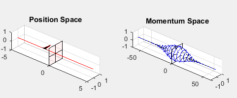
In the video:
There are two graphs present. One graph is the time evolution of a wavepacket in the position space, and the other graph is the time evolution of a wavepacket in the momentum space. The plane in the middle is at x = 0 and k = 0.
When the wavepacket moves along x, with either more positive or more negative x values, the wavepacket in the momentum space develops more kinks. The opposite relationship is also true, as when k values increase in the momentum space, the helix in the position space also gets kinkier. The handedness of the helices are based on the sign of k or x.
Position and momentum are still defined by their uncertainties relative to each other, where $ ΔxΔp≥ℏ/2 $.
If the position of a particle is known, the momentum will be more uncertain. If the momentum is well-defined, the position will not be well-defined. This relation hold true with gaussian wavepackets in postion and momentum space as well. If the wavepacket is narrow in position space. When the wavepacket in the position space is wide, the wavepacket in the momentum space evolves more slowly.
The Fourier transform is a linear combination of sines and cosines. The evolving combination of sines and cosines is what causes the helical shape, and with higher energy, higher k values, the helical shape will appear to evolve more quickly and display more kinks.
At a higher k values, the wavelength of the wavepacket will be decreased and the graph will appear more steep. At higher k values, or wavenumbers, the wavepacket will have more energy.